

Finding a good entry point, as discussed in a previous trading lesson, is often a key to investing success as many buy too high and then get stopped out before the market moves as they expect. This is often a result of focusing too much at the potential reward of a trade while paying too little attention to the risk.
When I am in a profitable trade I prefer to scale out of the position by selling on strength and in this trading lesson I will discuss how my exit price levels are determined for any market.
Those who have read my previous articles know that I prefer to come up with price levels using several different methods. Price targets are often determined by using a combination of pivot resistance levels, starc bands, Fibonacci projections and chart targets.
For example, the Spyder Trust (SPY) traded below its daily starc- band from November 1st through November 4th of 2016 as it had a low of $208.38. This was just below the 4th quarter pivot support at $209.04 but SPY held above the 50% support from the June low at $208.08.
On November 3rd, the iShares Russell 2000 (IWM) had a low of $114.88 which was just below the daily starc- band at $114.90. The quarterly pivot support at $115.72 was violated for three days in a row but IWM held above the 61.8% support from the May low at $114.14.
On October 3rd the SPDR S&P Regional Banking ETF (KRE) was recommended to Viper ETF clients at $41.90 based on the bullish readings from the weekly relative performance and OBV. At the time I certainly was not expecting the powerful rally in KRE that developed after the election.
By Thanksgiving week KRE was trading above the weekly starc+ band for the 3rd week in a row which meant it was in a high-risk buy area. It had also exceeded the quarterly pivot resistance levels. In some instances it is the past price performance of an ETF that will often tell one what type of gain can typically be expected.
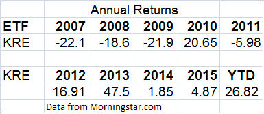
This yearly performance data reveals that KRE had its best annual return of 47.5% in 2013 as well as a return of 20.65% in 2010. There have only been three years so far with double-digit returns though it is already up 26.82% YTD in 2016.
Prior to the open on November 21st investors had an open profit of 22.9% in KRE so investors were advised to sell at $51.86 (a new high) which was hit the next day (see tweet). Even though the KRE has gained an additional 3.5% since longs were sold I continue to believe this was the right strategy.
Sector ETFs like the Energy Sector Select (XLE) often have strong trends that last 6 to 10 months but sometimes rallies or declines only last 2-3 months. Before the eighteen-month slide in crude oil and energy stocks XLE had a strong rally that started in the spring of 2014.
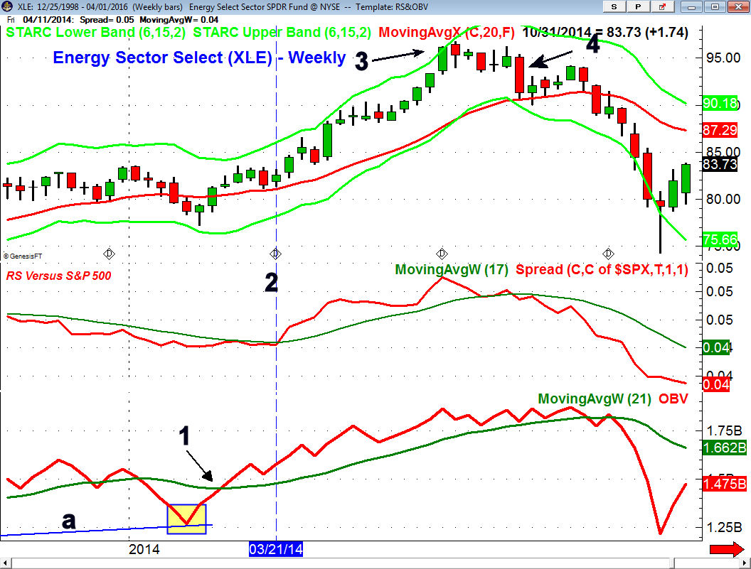
For the first six weeks of 2014 XLE was correcting as the OBV dropped to test the long term uptrend, line a. Just three weeks later the OBV moved back above its WMA (point 1) as volume had contracted on the decline and then expanded on the rally.
After moving above its 20 week EMA, XLE consolidated for two weeks before it dropped back to the 20 week EMA and the monthly pivot at $81.15. The next week the relative performance, which measures the performance of XLE versus the S&P 500, crossed back above its WMA (line 2). That indicated it was now leading the market higher.
The following week XLE pulled back to the buy point at 1/3 of the prior week's range at $82.68 with a weekly low of $82.26. XLE continued higher until the end of the week as it broke through the weekly resistance at $83.57. A stop under the low from the week after the correction low limited the risk to 5%.
The width of the weekly trading range was $7.18 so the upside target from the chart formation was in the $90-$91 area. A month later XLE had reached the weekly starc+ band as it traded above $90 before consolidating for five weeks. The average yearly gain of XLE over the past five years was just over 11%. Traders who took partial profits at $90 banked a 6.8% gain in six weeks.
Since the OBV was moving higher as XLE moved sideways there were no signs of a major top and by early June XLE had clearly broken out of its weekly range though was still well below the weekly starc+ band.
By June 20th XLE closed at $96.16 (point 3) which was well above both the weekly and monthly starc+ bands at $94.40 and $94.06 respectively. There were no signs of top from the daily studies but XLE was above its daily starc+ band which was another sign that risk on the long side was quite high.
Though a move to the weekly R1 at $97.20 was possible it is never a good idea to be greedy. Over the years I have occasionally made the mistake of holding out for my maximum upside target only to see the market reverse before the price target is reached.
Selling XLE on Monday's open turned out to be the best strategy as it opened higher at $96.47 but then reversed and closed the day at $94.49. It did not break weekly support at $93.50 until five weeks later (point 4)
One very effective strategy in buying stocks or ETFs is to find one that has had a weekly correction with a very bullish monthly chart and technical studies. The was the case in my recommendation of Walt Disney on February 3rd 2014.
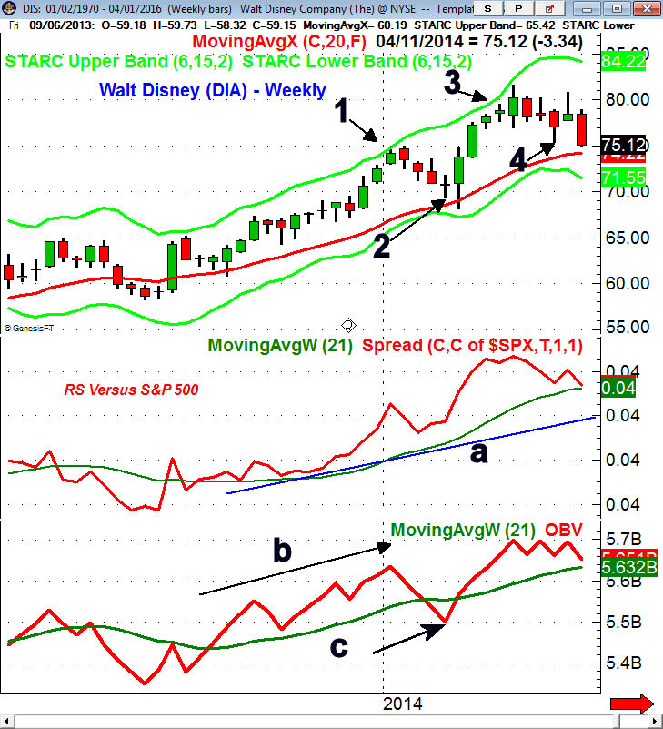
DIS had reached its weekly starc+ band in early January (point 1) before a four week pullback that ended in the formation of a doji. The relative performance analysis was strong as it was making sharply higher highs (line a) and this confirmed the monthly analysis that DIS was a market leader. The OBV had confirmed the highs in early January (line b) but did drop below its WMA on the correction, point c.
The initial buy was just above the doji low at $69.68 and the second buy level was at $68.55 with a stop at $66.59. On February 3rd DIS dropped below the 20 week EMA at $69.01 and reached a low of $68.14 before it reversed to the upside closing the week above the doji high.
The average price on the long positions was $69.11 and my original target was in the $78 to $80 area as the monthly starc+ band was at $81.14. In late February DIS appeared to be losing upside momentum so I recommended selling 1/3 of the position at $78.53 for a 13.6% profit.
At the time I thought that DIS would move even higher but I wanted to reduce the exposure by locking in a nice profit on part of the position. DIS made another push to the upside in early March hitting a high of $81.60 before it reversed. There were no divergences at the highs but the stop was raised to just under the last major swing low and the remaining position was stopped out at $76.73. The overall profit was 11.9%.
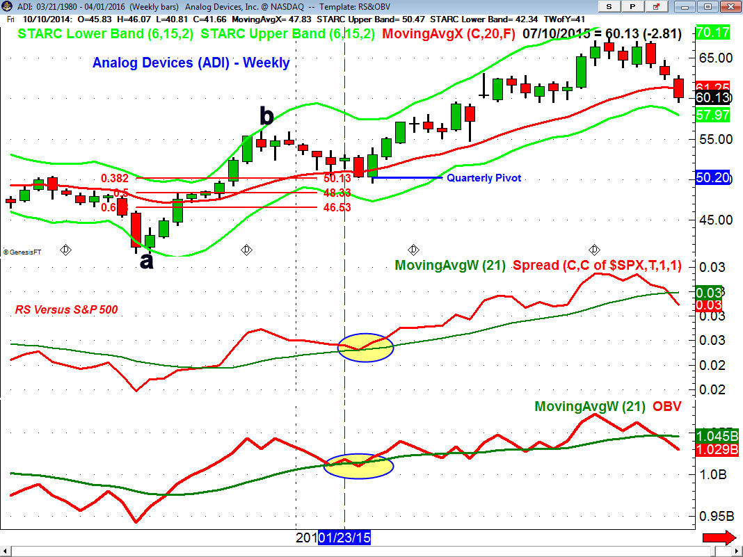
In a January 22, 2015 review of technology stocks I recommended Analog Devices (ADI). At the time I noted that after a nine week rally from the mid-October lows (point a to point b) ADI had corrected 5.9% over a six week period.
The decline had dropped ADI close to the quarterly pivot as well as the 38.2% retracement support of the rally from a to b. Both the RS and OBV analysis had given strong buy signals on the prior rally and had just pulled back to their WMAs.
As I noted in my trading lesson on entry techniques corrections often terminate between the 38.2% and 50% support levels. The fact that the quarterly pivot coincided with the 38.2% support was further confirmation that this was an important level of support.
The recommendation was to buy on a test of the previous low but I also would be buying a marginal new correction low when others were being stopped out. Seven days after the column was posted ADI hit a low of $49.51. Therefore the recommendation to go 50% long at $50.88 and 50% long at $50.16 were both filled. The stop at $47.88 was below the 50% retracement support at $48.33.
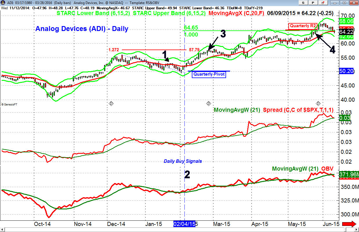
The daily chart shows that just a few days after the low the daily studies moved firmly back into the buy mode (line 2). Based on the correction from the December high to the early February low the 127.2% Fibonacci retracement target was at $57.79 and this was my initial upside target. Therefore 50% was sold just below this target at $57.47 (point 3) for a 13.7% profit is just three weeks.
The longer term targets were based on both Fibonacci and pivot point analysis. If the rally from the February low was equal to the rally from the October 2014 low (point a) to the December high (point b) then the equality target (in green) was at $64.95. The quarterly R1 resistance at $59.44 was exceeded in March so the stop was raised and the focus turned to the R2 resistance at $65.28.
On May 20th ADI moved above the daily starc+ band at $64.96 and closed at $64.31. Therefore I recommended taking profits at $64.82 or better as ADI was close enough to the converging target zones. The stop was also moved up in case of a reversal. The sell level was hit two days later and subsequently ADI hit a high of $67.43 in early June before it started a major correction.
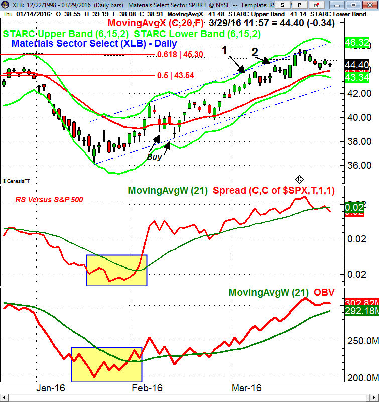
On February 8th 2016 I shared the following analysis in the Viper ETF Report "The weekly chart of XLB shows that it closed last week above the doji high from two weeks ago. As XLB made lower lows (line b) the OBV formed higher lows, line c. This bullish divergence is consistent with an important low."
The recommendation was for investors and traders to go 50% long XLB at $39.44 or better and 50% long at $38.59 with a stop at $36.92 (risk of 5.3%). The daily RS and OBV analysis had turned positive in early February so a setback was a buying opportunity consistent with the bullish weekly signals. The second buy level was hit at the February 11th low of $38.34 and XLB formed a doji. On the next day XLB generated a doji buy signal.
From the long term chart of XLB the major 50% retracement resistance from the February 2015 high was at $43.54 with the 61.8% resistance at $45.30. The midpoint between these resistance level was at $44.42. The daily chart shows a well defined trading channel with resistance from late 2015 in the $43-$44 area.
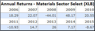
According to Morningstar the average yearly performance for XLB since 2006 was just over 11%. Other than a gain of 48.17% in 2009 a gain of over 10% in three weeks was much greater than could normally be expected. Though technically the rally was intact a significant pullback can never be ruled out. Therefore on March 4th traders sold 50% at $43.24 for a profit of 10.8%.
After a couple of day pullback XLB again moved higher and traders sold out the remaining position at $44.03. In order to reduce the risk on the position investors also sold 50% of their long position at $44.03 for a 12.8% profit.
I hope these examples have given you some insight on how I use Fibonacci, starc bands, pivot analysis as well as the charts to determine the price levels where you should consider exiting a position. I find that when you can determine a profit taking level, using a number of different methods, it can give you a greater degree of confidence.
Trying to get out at the top of a market is a fool's game as if you can capture 70-80% of a market's rally you will succeed in the long run. Once you have determined your profit targets you should actually place your order under your price targets. For example, if you have targets at $38.46 and $34.90 I would typically use an exit level at say $38.18 to $38.26.
The goal of these trading lessons is not only to give you a better understanding of the methods that I use in generating my analysis but also to hopefully give you additional insights on how the markets really work. I hope this will help you become a better investor and trader.
New Trading Lessons are sent on regularly to subscribers of either the Viper ETF Report and the Viper Hot Stocks Report. Reports are sent out twice a week and each service is just $34.95 per month and can be cancelled on line at any time. Four of the most recent trading lessons are also sent out to all new subscribers.
Comments
comments