

As I discussed in an earlier trading lesson on I use a combination of weekly relative performance, on-balance-volume and momentum to come up with a list of ETFs or stocks that I think that are likely to move higher or lower. Once a list has been assembled then the next step is to determine a good risk/reward entry level where the risk can be well managed.
In this lesson I would like to share some of the techniques that I use to determine good entry levels for ETFs like the Spyder Trust (SPY) or individual stocks. The first technique is based on the weekly price range of the previous period and is very simplistic requiring only a calculator.
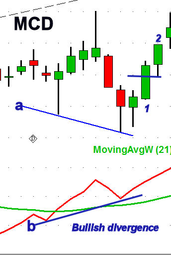
In the first example, the strong close at (point 1) put McDonalds Corp (MCD) on my buy list. The weekly on-balance-volume (OBV) had formed higher highs (line b) while prices had made lower lows, line a. The bullish divergence in the OBV was a sign that MCD was bottoming.
The weekly range in MCD was $90.86 to $88.44 or $2.42. One of the simplest methods is to base the initial entry on the week's range. If the weekly close is strong I use 1/3 of the range , in this case $0.80 is then subtracted from the high for an initial entry of $90.06. The following Monday MCD had a low of $89.91 before closing the week at $91.92 (point 2). Over the next three weeks it continued to make higher highs as well as higher lows surpassing the $95 level.
The second example is of Public Storage (PSA) which had corrected over a four week period. At point 1 PSA closed at $205.51 which was above the previous two week highs. The OBV that week reversed back above its WMA which was a bullish buy signal.
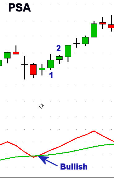
The range that week was $209.26-$199.32 for a range of $9.94 with PSA closing at $205.51. The weekly close was well under the week's high so a lower initial buy point was warranted than with MCD. Thus 50% of the week's range was $4.97 which when subtracted from the week's high of $209.26 gives you a buy price of $204.29.
Using a stop under the correction low meant a risk of 5.3%. PSA had a low for the next week at $203.19 and then closed at $207.78 (point 2). The following week PSA surged to close at $214.68 and by the end for
the year had surpassed the $250 level. It was not until seven weeks after the buy point that PSA had a lower weekly low.
Buying after a stock or ETF has completed a weekly flag or continuation pattern can often lead to the best profit opportunities.
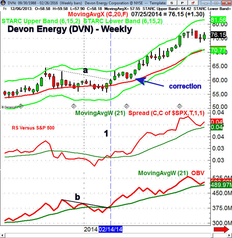
Devon Energy (DVN) peaked in October 2013 above the weekly starc+ band as it hit a high of $64.38. Over the next 15 weeks DVN corrected down to the major 61.8% support level. On February 7th it closed above the doji high from two weeks earlier and was on my buy list.
The relative performance signaled that DVN was now turning into a market leader as it had moved above its WMA
The weekly OBV was just breaking its downtrend, line b, and rallied to its WMA as the volume was supporting prices.
One of the other factors that I examine is the price ranges of the prior weeks. The close in DVN $58.92 was just above the prior three week high of $58.70 and also above the doji high of $57.63.
When a market closes near the week's high like DVN then it makes a strong opening more likely the following week.
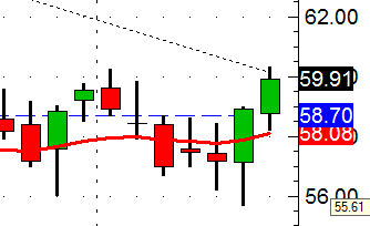
The 20 week EMA was at $57.89 and the mid-point between it and $58.70 (weekly support) was at $58.30. An initial buy level at $58.32 was reasonable. A stop would have needed to be under the weekly low at $55.68 as this low was below the lows of the prior eight weeks and likely triggered many stops. This would have meant a risk of 4.5%.
Based on the weekly price range of $59.00 to $55.68 was a range of $3.32 so 1/3 of the range was $1.10 which would have meant an entry level of $57.90. As it turned out the next week the low was $58.22 so the entry based on the weekly chart and 20 week EMA would have been filled but DVN never made it to the entry based on 1/3 of the weekly range.
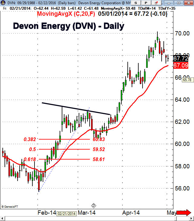
In a strongly trending market there are often many opportunities to buy or sell. In the case of DVN it surged from the weekly close at $58.92 to a high of $63.38 a week later as the daily starc+ band was exceeded.
DVN then began its correction but those who bought the first pullback were likely stopped out two weeks later as the initial correction low was violated. Traders are often stopped when they but the first pullback.
A safer strategy is to target a lower buying zone using a combination of Fibonacci retracement analysis, pivot levels and the 20 day EMA.
Based on the February low, the 38.2% support level was at $60.43 with the 50% support at $59.52. The key 61.8% level was at $58.61 and stops needed to be placed under this level. The monthly pivot point was at $60.42.
In this situation I will typically place my first buy level above the 38.2% support. In this case it was at $60.66 and the second level buy level is placed midway between the 38.2% and 50% support level at $59.98. As it turned out the low was $60.43 and at the monthly pivot.
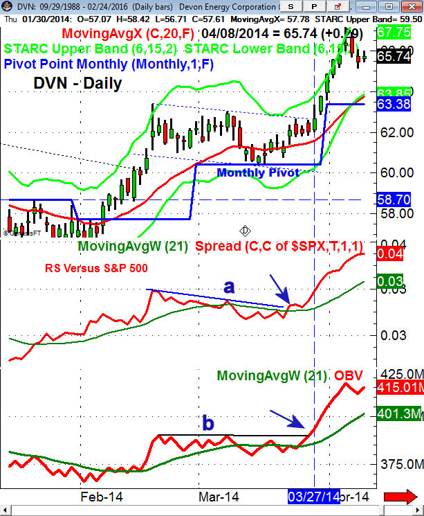
From the weekly chart it was clear that the technical studies had stayed positive through the correction.
The daily RS analysis moved through resistance (line a) and above its WMA five days after the lows. After a slight pullback it began to rally sharply. The OBV broke out of its trading range several days later (line b) as volume was confirming prices.
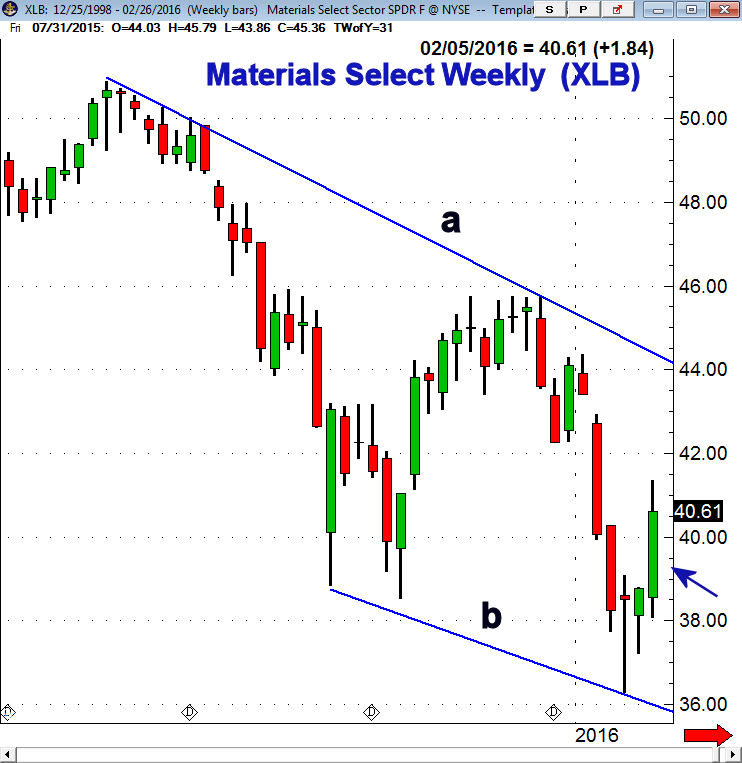
The bullish signals from my relative performance and OBV analysis put the Materials Sector Select (XLB) on my buy list in early February. XLB had also closed the week above the doji high at $39.08 from two weeks earlier.
The weekly chart revealed that the long term downtrend, line a, was in the $44 area.
After looking at the weekly chart the next step is to more closely examine the daily chart.
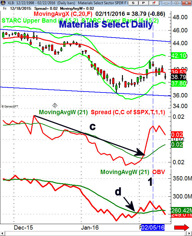
From the daily chart it is evident that XLB had reached the daily starc+ band on Thursday and then closed a bit lower with a narrow range on February 5th (line 1)
The 20 day EMA was at $39.56 with the daily starc- band at $37.61.
The downtrend in the daily relative performance, line c, was overcome in early February signaling that XLB was leading the S&P 500.
The RS line subsequently rallied sharply and by the end of the week was well above its rising WMA.
The daily OBV moved above its WMA in late January, point d, which was a positive sign. This was also consistent with the bullish divergence in the weekly OBV.
Though the daily OBV did drop back below its WMA on the correction but the weekly analysis is always more important .
On the 60 minute chart of XLB I have highlighted the trading on February 4th as XLB surged well above its starc+ band in the first hour of trading on and made its high at $41.35 in the next hour.
From the low on January 20th at $36.29 to this high one can then calculate the Fibonacci retracement levels for the rally. The 38.2% retracement level was at $39.43 with the 50% level at $38.84. XLB initially dropped to a low of $39.01 and between the retracement levels before it rebounded.
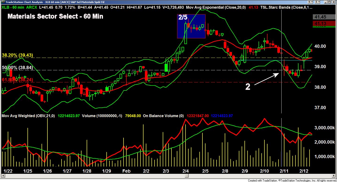
XLB then rallied up to a high of $41.22 before the correction resumed. On this decline XLB dropped below the 60 min starc- band (point 2) and eventually hit a low of $38.47 on February 11th. This was just above the 61.8% Fibonacci retracement support at $38.24.
Based on the weekly high and low of $41.35-$38.08 the range was $3.27. The 50% entry level was therefore at $41.35- 1.63 or at $39.71. The buy levels from the Viper ETF Report were 50% at $39.44 (38.2% support) and then 50% at $38.59.
Three days later XLB surpassed the high from the week of February 5th which was a sign that the correction was indeed over.
The entry approach is of course dependent on the type of signal you are following as well as the most recent price behavior. A majority of my recommendations are based on the weekly data . Occasionally the signals are so strong that more aggressive buying strategy is warranted.
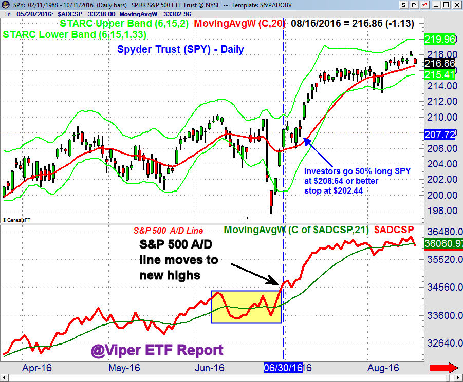
That was the case in early July just after the Brexit vote as the S&P 500 Advance/Decline line did not make a new low when the Spyder Trust (SPY) dropped to a low of $197.55 on June 27th. Just three days later the A/D line broke out to the upside as it overcame the highs from earlier in the month, line a.
The SPY held firm when the market reopened the following Tuesday July 5th but only had a low of $206.02 so our buy level at $204.74 was not hit. The very strong action of the A/D was a sign that stocks had a high probability of accelerating to the upside. Therefore on Thursday July 7th I recommended that "Investors go 50% long SPY at $208.64 or better with a stop at $202.44." The SPY traded as low as $207.58 and the next day SPY accelerated to the upside.
I hope this discussion of entry levels will help you become a better investor and trader. In a subsequent trading lesson I also reviewed the methods that I use to determine selling levels. These Viper Trading Lessons are sent on regularly to subscribers of either the Viper ETF Report and the Viper Hot Stocks Report. Reports are sent out twice a week and each service is just $34.95 per month and can be cancelled on line at any time. Four of the most recent trading lessons are also sent out to all new subscribers.
Comments
comments